Linear functions: manipulate the graph of f(x) = mx + n using slope and y-intercept; increasing–decreasing–constant, intercepts, sign; taxi fare model and catch the target lines
Interactively explore the changes of the equation f(x) = mx + n on the graph with the linear functions simulation. Easily learn increasing, decreasing, and constant function properties by seeing how the slope and y-intercept affect the graph.
What can you do in this simulation?
You can observe the movement of the line by changing the slope and the y-intercept.
You can examine the intercepts on the graph.
You can complete the 4 catch all target lines task.
You can test situations where the line is steeper or flatter.
You can answer questions with the guidance of the mentor and test your predictions with the experiment.
Basic concepts and formulas
Linear functions are expressed in the form f(x) = mx + n. Here, m represents the slope of the line, and n represents the y-intercept. If the slope is positive, the function is increasing; if negative, it is decreasing. The equations x = 0 and f(x) = 0 are used for the intercepts.
How to use?
Open the experiment panel and follow the guide.
Adjust the slope and y-intercept values using the sliders.
Observe the changes in the graph and the intercepts.
Find and check the correct parameters to catch the target lines.
Frequently asked questions
How does the slope value m affect the graph?
As the slope m increases, the line becomes steeper; as m decreases, it flattens, and for negative values, the function takes on a decreasing property.
What does the y-intercept n represent?
The y-intercept n determines the point (0, n) where the line intersects the y-axis, allowing the graph to shift up or down on the vertical axis.
How are the intercepts found?
To find the y-intercept, substitute 0 for x; to find the x-intercept, solve the equation f(x) = 0.
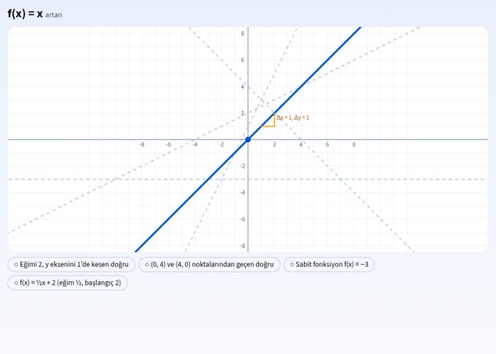 Interactive experiment